Chapter 12
Electromagnetic Induction
Maharashtra HSC · 13 subtopics · textbook pages 265–287
Formula SheetEvery formula this chapter can be examined on, in one table.
Constants, units and conventions
- Permeability of free space . The core of every coil in this chapter is air unless the question says otherwise.
- Magnetic flux is in weber (Wb), . Induced emf is in volt, and is in weber per second.
- Inductance and are in henry (H): .
- Angular frequency in . A speed given in r.p.m. must be divided by 60 to get in revolutions per second (Hz).
- Flux linkage of a coil of turns is , also in weber. For a closely wound coil every turn links the same flux.
- Every formula below is written for magnitudes; the minus sign in Faraday's law is Lenz's law and fixes only the direction.
Faraday's laws of electromagnetic induction
| Formula | Symbols, units and conditions |
|---|---|
| |
| |
| |
|
Flux of the field
| Formula | Symbols, units and conditions |
|---|---|
| |
| |
| |
| |
|
Motional electromotive force
| Formula | Symbols, units and conditions |
|---|---|
| |
| |
| |
| |
|
Induced emf in a stationary coil in a changing magnetic field
| Formula | Symbols, units and conditions |
|---|---|
| |
| |
| |
|
Generators
| Formula | Symbols, units and conditions |
|---|---|
| |
| |
| |
|
Induction and energy transfer
| Formula | Symbols, units and conditions |
|---|---|
| |
| |
|
Self inductance
| Formula | Symbols, units and conditions |
|---|---|
| |
| |
| |
| |
| |
| |
| |
| — | |
|
Energy stored in a magnetic field
| Formula | Symbols, units and conditions |
|---|---|
| — | |
| |
|
Energy density of a magnetic field
| Formula | Symbols, units and conditions |
|---|---|
| |
|
Mutual inductance
| Formula | Symbols, units and conditions |
|---|---|
| |
| — | |
| |
| |
| |
|
Transformer
| Formula | Symbols, units and conditions |
|---|---|
| |
| |
| |
|
Short NotesThe chapter subtopic by subtopic, in the textbook's own order.13 subtopics
- 1Introduction
- 2Faraday's Laws of Electromagnetic Induction2 board questions
- 3Lenz's Law2 board questions
- 4Flux of the Field
- 5Motional Electromotive Force5 board questions
- 6Induced emf in a Stationary Coil in a Changing Magnetic Field3 board questions
- 7Generators1 board question
- 8Back emf and back torque
- 9Eddy Currents1 board question
- 10Self Inductance1 board question
- 11Energy Stored in a Magnetic Field1 board question
- 12Mutual Inductance (M)5 board questions
- 13Transformer6 board questions
The whole chapter in brief
12.1 Introduction
- Electromagnetic induction is the phenomenon of producing an induced emf in a conductor or conducting coil because of a changing magnetic flux. Discovered by Faraday (1831); Joseph Henry demonstrated the same effect independently in the same year.
- Faraday's experiments with a bar magnet and a coil connected to a galvanometer (G):
- A magnet approaching the closed coil produces a current in it (the induced current); taking the magnet away produces a current in the opposite direction.
- Moving the coil instead of the magnet gives the same effect — only relative motion matters.
- Reversing the polarity of the moving magnet reverses the induced current.
- The magnitude of induced current depends on the relative speed of coil and magnet and on the number of turns of the coil.
- The induced current exists only so long as there is relative motion.
- Two-coil experiment: a primary coil with battery, rheostat and key faces a secondary coil connected to a galvanometer.
- A momentary deflection appears at make and at break of the primary circuit, in opposite directions.
- Relative motion between the two closed coils induces a current in the secondary as long as the motion lasts.
- Changing the primary current with the rheostat also deflects the galvanometer, for as long as the current is changing.
- Conclusion: whenever the flux through a coil changes — by a magnet or by a current-carrying coil — an emf is induced, and its direction reverses when the flux decreases instead of increasing.
12.2 Faraday's laws of electromagnetic induction
- First law (qualitative): whenever there is a change of magnetic flux in a closed circuit, an induced emf is produced in the circuit. Also, if a conductor cuts the lines of magnetic field, an emf is induced between its ends.
- Second law (quantitative): the magnitude of the induced emf produced in the circuit is directly proportional to the rate of change of magnetic flux linked with the circuit.
- Mathematically , so ; with all quantities in the same system of units , giving and, with Lenz's law, .
- For turns each linking flux , the total flux is and . This is the flux rule.
- SI: in volt, in weber per second.
- A moving magnet (a time-varying magnetic field) exerts a force on the stationary charges inside a conductor — this is the converse of a current exerting a force on a magnet.
12.3 Lenz's law
- Statement: the direction of the induced current in a circuit is such that the magnetic field produced by the induced current opposes the change in the magnetic flux that induces the current. The direction of the induced emf is the same as that of the induced current.
- Short form: the induced emf tends to set up a current whose action opposes the change that causes it. "Every effect of induction acts in opposition to the cause that produces it."
- Magnet approaching a loop: the loop develops a north pole facing the approaching north pole so as to repel it; the induced current is anticlockwise as seen from the magnet side. When the magnet is pulled away, the loop develops a south pole to attract the retreating north pole and the current reverses to clockwise.
- Jumping-ring experiment: a metal ring sits on the iron core of a vertical coil; when the current is switched on, the sudden upward flux induces a current in the ring opposite in direction to the coil current, opposite currents repel, and the ring flies into the air.
- Energy conservation: if the induced current helped the change that produced it, the current and the flux would grow without limit, giving Joule heating for free — a perpetual motion machine. Lenz's law is therefore a necessary consequence of the law of conservation of energy.
- Two cases of opposition — (i) a conductor moving in a field: the thrust on it from the field is opposite to its motion; (ii) a stationary circuit in a changing field: the induced current sets up a field opposite to the original field if that field is increasing, and in the same direction as it if it is decreasing.
- It is the change in flux, not the flux itself, that is opposed.
- For an open conductor, mentally complete the circuit, apply Lenz's law, and the polarity of the free ends follows.
- The negative sign in is exactly Lenz's law written into Faraday's law: it says the emf opposes the change of flux linked with the coil.
12.4 Flux of the field
- Give a small element of area a direction: if the bounding curve is traversed in the sense of the arrow, the normal comes out towards the reader — the right-handed screw rule.
- , where is the angle between and the assigned direction of .
- Over a finite surface , . can be pulled out of the integral only when it is the same at every point of .
- If the field varies with time, , and Faraday's law reads .
- The rate of change of flux equals the work done in taking unit positive charge once round the bounding contour in the reverse sense — that work is the emf.
- Even if is constant in time, the flux still changes if the area changes — this is the source of motional emf.
- SI: in volt, in weber, in second.
12.5 Motional electromotive force
- Translation: a rod of length slides on a C-shaped frame with velocity , increasing the enclosed area. , so .
- The same result from the Lorentz force: a charge in the moving rod feels , which is parallel to the rod; the work done over the length is , so , and when .
- The two routes — flux rule and Lorentz force — agree. In general, for any circuit whose parts move in a fixed field, the induced emf is the time derivative of the flux, whatever the shape of the circuit.
- The flux rule also holds when the loop is stationary and the field changes. Then the force on the charges comes from the term of : in a region where the magnetic field is changing with time, electric fields are generated, and it is this electric field that drives the current.
- Rotating bar: an element at distance from the pivot moves with and contributes ; the elements are in series, so . Compare with for a sliding bar.
- Faraday disc dynamo: a disc of radius spinning at in an axial field gives between rim and axis.
12.6 Induced emf in a stationary coil in a changing magnetic field
- Apparatus: a bar magnet mounted on an arc of a semicircle of radius 50 cm, part of a rigid aluminium frame suspended at the centre of the arc so the whole system swings freely in its plane. A coil of about 10000 turns of copper wire loops the arc so the magnet passes through it freely.
- Measurement: a capacitor and a diode are connected across the coil; the induced emf charges the capacitor through the diode and the voltage across is measured. Because the time constant can exceed the duration of the emf pulse, several oscillations may be needed; a milliammeter shows when the charging current stops, i.e. when the peak has been reached.
- The field at the coil is appreciable only when the magnet is near it, and the magnet is fastest at the mean position, so against is a hump 'bcde' whose flat top 'cd' corresponds to the finite length of the magnet.
- The induced emf is proportional to the slope of that curve. The slope is largest at (flux increasing) and (flux decreasing), so is largest there, and the minus sign makes negative at and positive at : one negative and one positive pulse in half a cycle, repeated on the return swing.
- Only the positive pulse is passed by the diode, so the capacitor charges in steps up to the peak .
- Writing with gives , and near the mean position the cosine is nearly 1, so .
- Result: for a given magnet-coil system, the peak emf is directly proportional to the angular amplitude and inversely proportional to the period .
12.7 Generators
- A generator has the same construction as a motor, but the armature is turned by an external torque instead of by a current. As the armature wires cut the lines of force, an emf appears across the terminals; it is proportional to the speed of rotation .
- Following one conductor of the armature: (i) moving up across the lines of force — emf maximum; (ii) moving parallel to the field — ; (iii) moving down across the lines — emf reversed; (iv) the graph of current against time is a sinusoid.
- For a coil rotating at constant , , , so with .
- swings between and , so the polarity reverses periodically: this is alternating current. The emf is extremum at and , where the flux changes fastest. Domestic supply is 50 cycles per second.
- A split-ring commutator reverses the connections to the armature in step with the reversals of the current, converting the AC waveform into pulsating DC — used for charging a storage battery.
- Modern AC motors are more compact and rugged than DC motors.
12.8 Back emf and back torque
- Emf can be produced in many ways: chemical force in a battery, mechanical pressure in a piezoelectric crystal, a temperature gradient in a thermocouple, light in a photoelectric cell, mechanical transport of charge in a Van de Graaff generator, and motion of a wire in a magnetic field in a generator.
- A DC generator and a DC motor are physically the same machine: connect a generator to a battery and it runs as a motor; turn a motor by an external agency and it acts as a generator. So a running motor cannot switch its generator action off.
- By Lenz's law the emf so induced opposes its cause — here the armature current — and therefore reduces it. This unavoidable emf is called the back emf.
- At start-up the armature is not turning, there is no back emf, and the current is large. As the motor speeds up, the back emf grows and the armature current falls. That is why the starting current of a motor is much larger than its running current.
- Application: in hybrid and electric vehicles the car acts as a generator while braking, and back emf is used to charge the battery for a longer drive.
12.9 Induction and energy transfer
- A rectangular loop of width and total resistance is pulled out of a uniform field region with constant velocity . The area inside the field, and hence the flux , decreases.
- Induced emf ; induced current , clockwise, with its direction given by the right-hand rule.
- Three segments of the loop are still in the field. The forces and on the two side arms are equal and opposite and cancel; the force on the leading arm opposes the motion, so the applied force must be in direction and in magnitude.
- , so the mechanical power is .
- The rate of Joule heating is — exactly the same.
- Conclusion: the work done in pulling the loop through the field appears entirely as heat energy in the loop.
12.10 Eddy currents
- Definition: the circulating currents induced in a metal block (a bulk conductor) when it is placed or moved in a changing magnetic field are called eddy currents.
- Replace the loop of 12.9 by a solid plate and the electrons no longer follow one path — they swirl within the plate like eddies in water. Work must still be done to move the plate, and that work becomes heat.
- Pendulum demonstration: a conducting plate free to swing about a pivot loses a part of its mechanical energy to heat each time it enters and leaves the field; after several swings it stops and the plate is warm.
- Reduction: cut slots in the plate (a discontinuous, laminated structure) so the eddy paths are broken.
- Applications the board accepts (any two):
- Dead beat galvanometer — the coil is wound on a light aluminium frame; eddy currents in the frame oppose its motion and bring the coil quickly to rest.
- Induction motor / speedometer — a magnet rotating at the vehicle's speed inside a spring-pivoted aluminium drum sets up eddy currents; the drum turns with the magnet and a pointer reads the speed on a calibrated scale.
- Electric (induction) brake — with the drive power off, a stationary magnetic field applied to the rotating drum sets up strong eddy currents whose torque opposes the rotation and stops the train quickly and smoothly.
- Induction furnace — a high-frequency alternating current in a coil around a crucible produces a rapidly varying field and very strong eddy currents whose heat melts the metal; used for making alloys in vacuum.
12.11 Self inductance
- The production of an induced emf in a circuit (coil) itself, because of a change of current in it, is called self-induction.
- , so and ; for a closely wound coil of turns the flux linkage is , so .
- depends only on the geometry of the coil and the material properties of its core.
- Three definitions the board accepts:
- The magnetic flux (linkage) produced per unit current in the circuit.
- The induced emf produced per unit rate of change of current: , since .
- Numerically twice the work done in establishing the flux associated with unit current: , so when .
- Unit: ; also .
- Solenoid: , so , and . Hence and , and can be written in .
- plays the same role in a circuit — electrical inertia — that mass plays in mechanics: compare with .
- Combinations: in series; in parallel.
12.12 Energy stored in a magnetic field
- The induced emf opposes the growth of current, so work must be done to build up the magnetic field; that work is stored in the field and can be recovered as heat in the resistance of the circuit.
- ; work done in moving charge against this emf is , using .
- Total work .
- Analogy with electrostatics: for a capacitor; for an inductor.
12.13 Energy density of a magnetic field
- For a solenoid of length and area , the energy is confined to the interior volume (the field outside is almost zero) and is uniformly distributed there.
- ; putting gives .
- With this becomes , in .
- This holds at any point where the field is , no matter how the field is produced. It parallels .
12.14 Mutual inductance
- Mutual induction: a change of current in one coil induces an emf in a neighbouring coil, through the flux it sends across.
- ; with the coils fixed in space , so and . Similarly and . By symmetry .
- Definitions: , the flux linked with the secondary per unit current in the primary; and , the emf induced in the secondary per unit rate of change of primary current. Also , the mutual potential energy for unit current in each.
- Unit: henry. if in the primary induces in the secondary; .
- Coefficient of coupling measures the fraction of coil 1's flux that reaches coil 2. Since , and , one gets .
- ; is perfect coupling and . tightly coupled, loosely coupled. If then for perfect coupling.
- is largest when the coils are coaxial (parallel and in line) and smallest when their axes are at right angles; two coils on a common iron core have ; radio-frequency coils have between 0.001 and 0.05.
- A large is wanted in a transformer but is dangerous in appliances: a clothes dryer has counter-wound heating coils so their fields cancel and no dangerous emf appears on the metal case.
- Why two coils in parallel have less inductance than either coil: in parallel the current through each inductor is only a fraction of the total, while the voltage across each is the same. A given rate of change of total current therefore develops less voltage across the array than across any single coil — and less voltage for the same means less inductance.
12.15 Transformer
- A transformer is an electrical device which converts low alternating voltage at high current into high alternating voltage at low current, and vice versa.
- Principle: mutual induction — whenever the magnetic flux linked with a coil changes, an emf is induced in the neighbouring coil.
- Construction: two coils, primary P (input) and secondary S (output), insulated from each other and wound separately on a laminated soft-iron core. In a step-up transformer .
- Working: an alternating voltage applied to P makes the primary current, and hence the flux in the core, change sinusoidally; this changing flux links both coils and induces an emf in each. The emf depends on the number of turns.
- With the flux per turn, and , so — the equation of the transformer; is the turns (transformer) ratio.
- For an ideal transformer input power equals output power: , so , and therefore .
| No. | Step-up transformer | Step-down transformer |
|---|---|---|
| i. | Turns in secondary more than in primary, | Turns in primary more than in secondary, |
| ii. | Alternating voltage across secondary more than across primary, | Alternating voltage across primary more than across secondary, |
| iii. | Transformer ratio | Transformer ratio |
| iv. | Primary coil made of thick wire | Secondary coil made of thick wire |
| v. | Secondary coil made of thin wire | Primary coil made of thin wire |
| vi. | Current through secondary less than through primary | Current through primary less than through secondary |
Self induction against mutual induction
| Point | Self induction | Mutual induction |
|---|---|---|
| Coils involved | One coil | Two neighbouring coils |
| Cause | Change of current in the same coil | Change of current in the neighbouring (primary) coil |
| Coefficient | ||
| Induced emf | ||
| Unit | henry | henry |
Traps that cost marks
- Induced emf depends on the rate of change of flux, not on the flux itself. A coil sitting in a huge steady field has zero induced emf.
- Forgetting the factor : for a coil of turns it is , and the flux linkage asked for in MCQs is , not .
- When a field is reversed (or a coil is flipped through ), the change of flux is , not . A search coil pulled fully out of the field, however, changes by .
- "Plane of the coil perpendicular to " means and ; "plane of the coil parallel to " means and . Read which is which before writing .
- only when , and are mutually perpendicular. In general with the angle between and — a wire lying east-west and falling vertically moves along , so and the emf is zero.
- Rotating rod: , with the factor ; the sliding rod has no such factor. In terms of revolutions per second, .
- Convert r.p.m. to in Hz by dividing by 60, and always use in . Writing loses the .
- is fixed by geometry and core material. It does not change when the current or the emf changes — a question giving and is asking you to compute , not claiming depends on them.
- Inductances combine like resistances, not like capacitances: series adds, parallel adds reciprocals.
- Energy stored is , not ; energy density is (per unit volume), not the total energy.
- with the square root; is a pure number never greater than 1, and "what percentage of the flux reaches the other coil" is asking for .
- The transformer equation has the current ratio inverted: . A step-up transformer raises voltage and lowers current; it never raises power.
- A transformer works only on AC. With DC the flux is steady, so no emf is induced in the secondary.
- Lenz's law opposes the change in flux, not the flux; and it follows from conservation of energy, which is what a question asking to "explain Lenz's law in the light of conservation of energy" wants.
- Eddy currents are currents in a bulk conductor, not in a wire loop; the standard answer names dead beat galvanometer, speedometer, electric brake and induction furnace.
- In numericals, work with magnitudes: the minus sign of Faraday's law is for direction only, so do not carry it into the arithmetic and then report a negative emf.
Solved Numerical ExamplesWorked numericals to attempt first, each with a hint before the full solution.Coming soon
These are being added chapter by chapter. They are solved numericals from the prescribed book and the reference guides — not previous board questions, which live under Practice — so that you can work through the method before meeting it in a real paper.
Important DerivationsEvery derive / obtain / prove question in this chapter. 1 have come up in two or more papers.4
- 1Motional emf induced in a straight conductor moving in a uniform magnetic fieldDerive an expression for emf (e) generated in a conductor of length (l) moving in a uniform magnetic field (B) with uniform velocity (v) along the x-axis.
Asked in: March 2022 (Q.20, 3 marks)
Show the derivationHide the derivation
Step 1Consider a C shaped frame of wires PQRS of area (lx) situated in a constant magnetic field . Here, QR is a conducting wire that slides on the frame parallel to PS.Step 2As the wire QR of length l is moved out with velocity to increase x, the area of the loop PQRS increases. Thus the flux of through the loop increases with time.Step 3According to the flux rule, the induced emf will be equal to the rate at which the magnetic flux through a conducting circuit changes.Step 4The induced emf will cause a current in the loop. It is assumed that there is enough resistance in the wire so that the induced currents are very small producing negligible magnetic field.Step 5As the flux through the frame PQRS is Blx, magnitude of the induced emf can be written aswhere v is the velocity of wire QR increasing the length x of wires PQ and SR.Step 6Now, a charge q which is carried along by the moving wire QR, experiences Lorentz force ; which is perpendicular to both and and hence is parallel to wire QR.Step 7The force is constant along the length l of the wire QR (as v and B are constant) and zero elsewhere ( v = 0 for stationary part RSPQ of wire frame).Step 8When the charge q moves a distance l along the wire, the work done by the Lorentz force iswhere = angle between and .Step 9The emf generated is,Step 10For maximum induced emf,Step 11Thus, from equation (1) and (2), for any circuit whose parts move in a fixed magnetic field, the induced emf is the time derivative of flux () regardless of the shape of the circuit.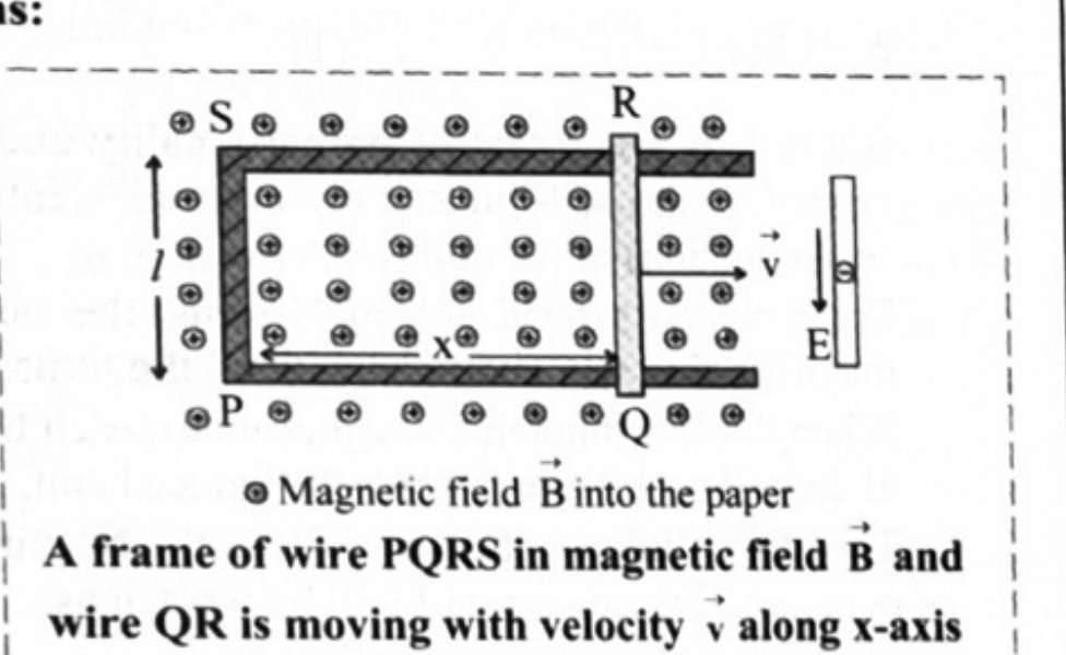
- 2Energy stored in the magnetic field in terms of induced currentDerive an expression for energy stored in the magnetic field in terms of induced current.
Asked in: February 2023 (Q.28(i), 4 marks)
Show the derivationHide the derivation
Step 1Changing magnetic flux in a coil causes an induced emf.Step 2The induced emf so produced opposes the change and hence the energy has to be spent to overcome it to build up the magnetic field.Step 3This energy may be recovered as heat in a resistance of the circuit.Step 4The induced emf is given as,Step 5The work done in moving a charge dq against this emf is,Step 6Therefore total work,Step 7Equation (1) gives the energy stored () in magnetic field and is analogous to the energy stored () in the electric field in a capacitor. - 3Transformer -- construction, working, and the transformer equation RepeatsExplain the construction and working of a transformer. Derive the equation for a transformer.
Asked in: March 2014; March 2016; July 2017; February 2024 (Q.27, 4 marks)
Show the derivationHide the derivation
Principle: Working of a transformer is based on the principle of mutual induction i.e., whenever the magnetic flux linked with a coil changes, an e.m.f is induced in the neighbouring coil.Construction:Step 1A step-up transformer consists of two sets of coils primary P and secondary S insulated from each other. The number of turns in secondary coil is greater than the number of turns in primary coil . The coil P is called the input coil and coil S is called the output coil.Step 2The two coils are wound separately on a laminated soft iron core.Step 1Construction:a. A transformer consists of two sets of coils primary P and secondary S insulated from each other. The coil P is called the input coil and coil S is called the output coil.b. The two coils are wound separately on a laminated soft iron core.Step 2Working:a. When an alternating voltage is applied to the primary coil the current through the coil goes on changing. Hence, the magnetic flux through the core also changes.b. As this changing magnetic flux is linked with both the coils, an e.m.f is induced in each coil.c. The amount of the magnetic flux linked with the coil depends upon the number of turns of the coil.d. Let, '' be the magnetic flux linked per turn with both the coils at certain instant 't'.e. Let '' and '' be the number of turns of primary and secondary coil,= magnetic flux linked with the primary coil at certain instant 't'= magnetic flux linked with the secondary coil at certain instant 't'f. Induced e.m.f produced in the primary and secondary coil is given by,g. Dividing equation (2) by (1),Equation (3) represents equation of transformer.The ratio is called turns ratio (transformer ratio) of the transformer.h. For an ideal transformer,Input power = Output powerStep 1From equation (3) and (4),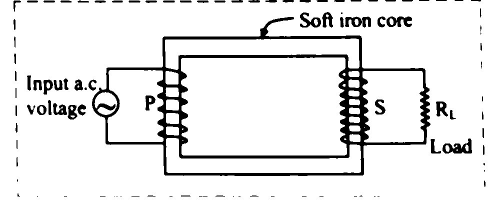
- 4Motional emf in a rotating bar (constant angular velocity, uniform field)Obtain an expression for motional e.m.f. in a rotating bar with constant angular velocity '' in a uniform magnetic field perpendicular to the plane of rotation.
Asked in: June 2025 (Q.29, 4 marks)
Show the derivationHide the derivation
The question is a real board question. This working is ours — no source printed a derivation for it.
Diagram
Draw a straight conducting bar of length pivoted at , rotating anticlockwise in the plane of the paper with constant angular velocity , sweeping out a circle of radius . Show the uniform magnetic field perpendicular to that plane by a grid of crosses (into the page). Mark a small element of the bar of length at a distance from the pivot , and the linear velocity of that element, drawn tangentially.
Method 1 — integrating the motional emf along the bar
Consider the small element of the bar of length at a distance from the pivot. Being rigidly attached, it moves with linear speed
Its velocity is tangential, and the field is perpendicular to the plane of rotation, so , and the element are mutually perpendicular. The motional emf across this element is
Different elements move at different speeds, so the emfs must be added by integrating from the pivot () to the free end ():
Method 2 — from Faraday's law (a useful check)
In time the bar sweeps out a sector of angle , of area
The flux through the swept area is , so by Faraday's law the magnitude of the induced emf is
the same result.
Notes
- Writing for rotations per second gives
.
- The emf is steady, not alternating: the bar sweeps area at a constant rate,
so the flux grows linearly and its rate of change is constant. The free end is at one polarity and the pivot at the other, the sign following from .
- The emf is proportional to , not to — doubling the length of the
bar quadruples the emf, because the outer parts of a longer bar also move faster.
Finished revising this chapter? Practise Electromagnetic Induction →