Graphical Representation of S.H.M.

Oscillations · Maharashtra HSC

Theory

Definition of linear S.H.M.

Linear S.H.M. is defined as the linear periodic motion of a body, in which force (or acceleration) is always directed towards the mean position and its magnitude is proportional to the displacement from the mean position.

Phase in S.H.M. (or for any motion) is the state of oscillation, given by $\theta=\omega t+\phi$ .

(a) Particle starting from the mean position, towards the positive

As the particle starts from the mean position, $\phi=0$ : $x=A\sin\omega t$ $v=\dfrac{dx}{dt}=A\omega\cos\omega t$ $a=\dfrac{dv}{dt}=-A\omega^2\sin\omega t$

$t$	$0$	$T/4$	$T/2$	$3T/4$	$T$	$5T/4$
$\theta=\omega t+\phi$	$0$	$\dfrac{\pi}{2}$	$\pi$	$\dfrac{3\pi}{2}$	$2\pi$	$\dfrac{5\pi}{2}$
$x$	$0$	$A$	$0$	$-A$	$0$	$A$
$v$	$A\omega$	$0$	$-A\omega$	$0$	$A\omega$	$0$
$a$	$0$	$-A\omega^2$	$0$	$A\omega^2$	$0$	$-A\omega^2$

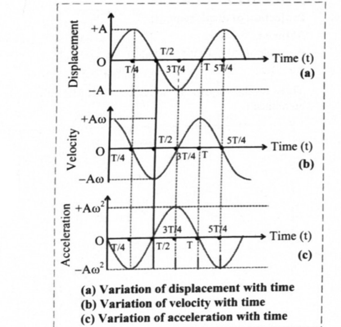
Graph (Fig. 5.6), three curves drawn one below the other against $t$ (or against the phase $\theta$ ) on a common time axis:

(a) Displacement against time: a sine curve starting at the origin, rising to $+A$ at $\dfrac{T}{4}$ , back to zero at $\dfrac{T}{2}$ , down to $-A$ at $\dfrac{3T}{4}$ and back to zero at $T$ .
(b) Velocity against time: a cosine curve starting at its maximum $+A\omega$ , zero at $\dfrac{T}{4}$ , minimum $-A\omega$ at $\dfrac{T}{2}$ , zero at $\dfrac{3T}{4}$ , back to $+A\omega$ at $T$ .
(c) Acceleration against time: an inverted sine curve — zero at $t=0$ , minimum $-A\omega^2$ at $\dfrac{T}{4}$ , zero at $\dfrac{T}{2}$ , maximum $+A\omega^2$ at $\dfrac{3T}{4}$ , zero at $T$ .

(b) Particle starting from the positive extreme position

As the particle starts from the positive extreme position, $\phi=\dfrac{\pi}{2}$ , so the phase is $\theta=\omega t+\dfrac{\pi}{2}$ and $x=A\sin\left(\omega t+\dfrac{\pi}{2}\right)=A\cos\omega t$ $v=\dfrac{dx}{dt}=\dfrac{d}{dt}(A\cos\omega t)=-A\omega\sin\omega t$ $a=\dfrac{dv}{dt}=\dfrac{d}{dt}\left(-A\omega\sin\omega t\right)=-A\omega^2\cos\omega t$

$t$	$0$	$T/4$	$T/2$	$3T/4$	$T$	$5T/4$
$\theta=\omega t+\phi$	$\dfrac{\pi}{2}$	$\pi$	$\dfrac{3\pi}{2}$	$2\pi$	$\dfrac{5\pi}{2}$	$3\pi$
$x$	$A$	$0$	$-A$	$0$	$A$	$0$
$v$	$0$	$-A\omega$	$0$	$A\omega$	$0$	$-A\omega$
$a$	$-A\omega^2$	$0$	$A\omega^2$	$0$	$-A\omega^2$	$0$

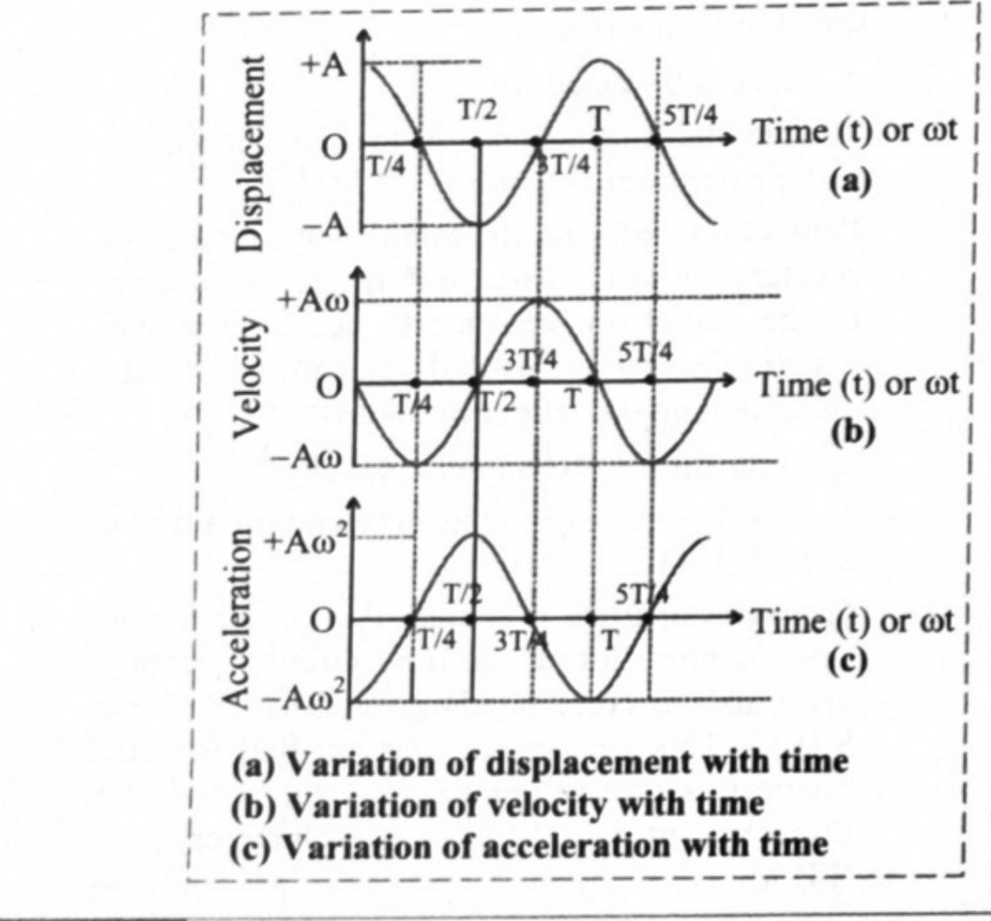
Graph (Fig. 5.7), again three curves on a common time axis:

(a) Displacement against time: a cosine curve starting at $+A$ , zero at $\dfrac{T}{4}$ , $-A$ at $\dfrac{T}{2}$ , zero at $\dfrac{3T}{4}$ , back to $+A$ at $T$ .
(b) Velocity against time: an inverted sine curve — zero at $t=0$ , minimum $-A\omega$ at $\dfrac{T}{4}$ , zero at $\dfrac{T}{2}$ , maximum $+A\omega$ at $\dfrac{3T}{4}$ .
(c) Acceleration against time: an inverted cosine curve — minimum $-A\omega^2$ at $t=0$ , zero at $\dfrac{T}{4}$ , maximum $+A\omega^2$ at $\dfrac{T}{2}$ , zero at $\dfrac{3T}{4}$ .

Conclusions from the graphs

Displacement, velocity and acceleration of S.H.M. are periodic functions of time.
For a particle starting from the mean position, the displacement–time and acceleration–time curves are sine curves and the velocity–time curve is a cosine curve.
There is a phase difference of $\dfrac{\pi}{2}$ radian between displacement and velocity.
There is a phase difference of $\dfrac{\pi}{2}$ radian between velocity and acceleration.
There is a phase difference of $\pi$ radian between displacement and acceleration — the acceleration curve is exactly the inverted displacement curve, which is the statement $a=-\omega^2x$ .
Shapes of all the curves get repeated after $2\pi$ radian, i.e. after a time $T$ .

Standard results

From the mean position: $x=A\sin\omega t$ , $v=A\omega\cos\omega t$ , $a=-A\omega^2\sin\omega t$
From the positive extreme: $x=A\cos\omega t$ , $v=-A\omega\sin\omega t$ , $a=-A\omega^2\cos\omega t$
Phase differences: $x$ and $v$ — $\dfrac{\pi}{2}$ ; $v$ and $a$ — $\dfrac{\pi}{2}$ ; $x$ and $a$ — $\pi$
Velocity is zero where displacement is maximum; acceleration is zero where displacement is zero

Theory Questions Asked on This Subtopic

Real board questions. Answers are at the end of the page.

1
Represent graphically the displacement, velocity and acceleration against time for a particle performing linear S.H.M., when it starts from the mean position.
Maharashtra HSC board question — asked in March 2008Answer 1 ↓
2
Give graphical representation of S.H.M. when particle starts from the positive extreme position.
Maharashtra HSC board question — asked in October 2009Answer 2 ↓
3
Define phase of S.H.M. Show variation of displacement, velocity and acceleration with phase for a particle performing linear S.H.M. graphically, when it starts from extreme position.
Maharashtra HSC board question — asked in October 2014Answer 3 ↓
4
Define linear simple harmonic motion. Assuming the expression for displacement of a particle starting from extreme position, explain graphically the variation of velocity and acceleration w.r.t. time.
Maharashtra HSC board question — asked in July 2017Answer 4 ↓

Answers & Solutions

Work the questions above first, then check yourself here. Each answer is set out the way it should be written in the paper.

1.↑ back to the question
Graph: (a) Variation of displacement with time (b) Variation of velocity with time (c) Variation of acceleration with time
2.↑ back to the question
Graph: (a) Variation of displacement with time (b) Variation of velocity with time (c) Variation of acceleration with time

3.↑ back to the question

Definition: Phase in S.H.M. (or for any motion) is the state of oscillation. Particle performing S.H.M., starting from the positive extreme position: Equations: As the particle starts from the positive extreme position, $\phi=\dfrac{\pi}{2}$ $\therefore$ Phase, $\theta=\omega t+\phi=\omega t+\pi/2$ $\therefore$ Displacement, $x=A\sin(\omega t+\pi/2)=A\cos\omega t$ Velocity, $v=\dfrac{dx}{dt}=\dfrac{d(A\cos\omega t)}{dt}=-A\omega\sin(\omega t)$ Acceleration, $a=\dfrac{dv}{dt}=\dfrac{d[-A\omega\sin(\omega t)]}{dt}=-A\omega^2\cos(\omega t)$ Table:

(t)	0	T/4	T/2	3T/4	T	5T/4
(θ)	$\dfrac{\pi}{2}$	π	$\dfrac{3\pi}{2}$	2π	$\dfrac{5\pi}{2}$	3π
(x)	A	0	−A	0	A	0
(v)	0	−Aω	0	Aω	0	−Aω
(a)	$-A\omega^2$	0	$A\omega^2$	0	$-A\omega^2$	0

Graph: [From 5.9, Q2] Graph: (a) Variation of displacement with time (b) Variation of velocity with time (c) Variation of acceleration with time

4.↑ back to the question

Definition: [From 5.4, Q2 (Definition only)] Definition: Linear S.H.M. is defined as the linear periodic motion of a body, in which force (or acceleration) is always directed towards the mean position and its magnitude is proportional to the displacement from the mean position. Differential equation of linear S.H.M.: [From 5.4, Q1]

i. In a linear S.H.M., the force is directed towards the mean position and its magnitude is directly proportional to the displacement of the body from mean position. $\therefore f\propto -x$ $\therefore f=-kx\qquad....(1)$ where, k is force constant and x is displacement from the mean position. ii. According to Newton's second law of motion, $f=ma\qquad....(2)$ From equations (1) and (2), $ma=-kx\qquad....(3)$ iii. The velocity of the particle is given by, $v=\dfrac{dx}{dt}$ , $\therefore$ Acceleration, $a=\dfrac{dv}{dt}=\dfrac{d^2x}{dt^2}\qquad....(4)$ iv. Substituting equation (4) in equation (3), $m\dfrac{d^2x}{dt^2}=-kx$ $\therefore \dfrac{d^2x}{dt^2}+\dfrac{k}{m}x=0$ v. Substituting $\dfrac{k}{m}=\omega^2$ , where ω is the angular frequency, $\therefore \dfrac{d^2x}{dt^2}+\omega^2x=0$ This is the differential equation of linear S.H.M. Variation of velocity and acceleration w.r.t. time: [From 5.9, Q3 (Velocity time graph and acceleration-time graph and explanation)] Definition: Phase in S.H.M. (or for any motion) is the state of oscillation. Particle performing S.H.M., starting from the positive extreme position: Equations: As the particle starts from the positive extreme position, $\phi=\dfrac{\pi}{2}$ $\therefore$ Phase, $\theta=\omega t+\phi=\omega t+\pi/2$ $\therefore$ Displacement, $x=A\sin(\omega t+\pi/2)=A\cos\omega t$ Velocity, $v=\dfrac{dx}{dt}=\dfrac{d(A\cos\omega t)}{dt}=-A\omega\sin(\omega t)$ Acceleration, $a=\dfrac{dv}{dt}=\dfrac{d[-A\omega\sin(\omega t)]}{dt}=-A\omega^2\cos(\omega t)$ Table:

(t)	0	T/4	T/2	3T/4	T	5T/4
(θ)	$\dfrac{\pi}{2}$	π	$\dfrac{3\pi}{2}$	2π	$\dfrac{5\pi}{2}$	3π
(x)	A	0	−A	0	A	0
(v)	0	−Aω	0	Aω	0	−Aω
(a)	$-A\omega^2$	0	$A\omega^2$	0	$-A\omega^2$	0

Graph: [From 5.9, Q2] Graph: (a) Variation of displacement with time (b) Variation of velocity with time (c) Variation of acceleration with time