Magnetic Field due to a Current: Biot-Savart Law

Statement of the Biot-Savart law

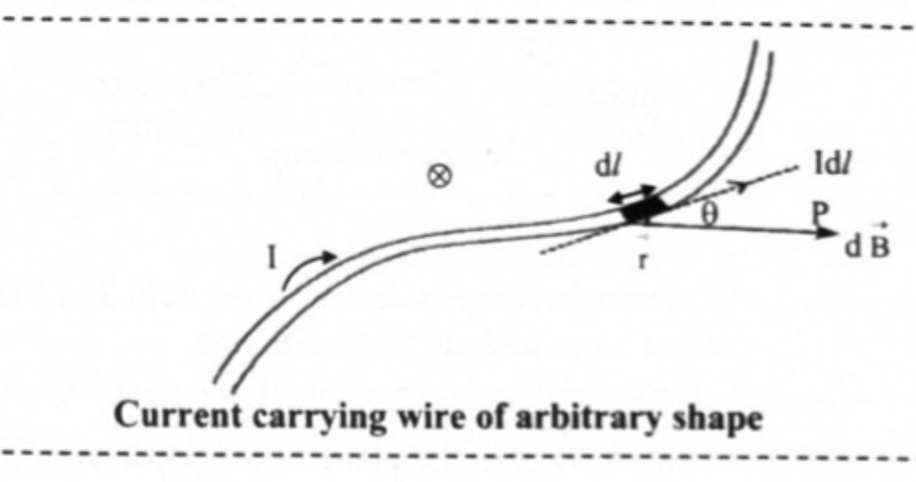
Diagram (Fig. 10.15): a wire of arbitrary shape carrying a current $I$. A short length element $d\vec{l}$ is marked on it, pointing along the current. A point P lies at a distance $r$ from the element, with $\vec{r}$ drawn from the element to P and $\theta$ the angle between $d\vec{l}$ and $\vec{r}$. The elementary field $d\vec{B}$ at P is marked with the symbol $\otimes$, indicating that it is directed into the plane of the paper.

The board's steps:

• Consider an arbitrarily shaped wire carrying a current $I$.
• Let $d\vec{l}$ be a length element along the wire; the current in this element is in the direction of the length vector $d\vec{l}$, and it produces a differential magnetic field $d\vec{B}$ at P.
• Let P be at distance $r$ from the element. The net field at P is obtained by superimposing, that is integrating, the fields $d\vec{B}$ from all the length elements along the wire.
• Experimentally, the magnetic field $d\vec{B}$ produced by current $I$ in the length element $d\vec{l}$ is

$$dB = \dfrac{\mu_0}{4\pi}\,\dfrac{I\,dl\,\sin\theta}{r^2}$$

where $\theta$ is the angle between the directions of $d\vec{l}$ and $\vec{r}$, and $\mu_0$ is the permeability of free space,

$$\mu_0 = 4\pi\times10^{-7}\ \text{T m/A} \approx 1.26\times10^{-6}\ \text{T m/A}$$

• The direction of $d\vec{B}$ is dictated by the cross product $d\vec{l}\times\vec{r}$. Vectorially,

$$d\vec{B} = \dfrac{\mu_0}{4\pi}\,\dfrac{I\,d\vec{l}\times\vec{r}}{r^3}$$

These two equations are the Biot-Savart law. It is an experimentally deduced inverse square law — the $r^3$ in the denominator is compensated by the one power of $r$ carried by $\vec{r}$ in the numerator.

The Biot-Savart law plays the role in magnetostatics that Coulomb's law plays in electrostatics.

Application 1: current in a straight, long wire

Diagram (Fig. 10.16): a long straight wire carrying current $I$ upward in the plane of the paper. P is a point at perpendicular distance $R$ from the wire. A current element $d\vec{l}$ at a distance $l$ along the wire from the foot of the perpendicular is joined to P by $\vec{r}$, with $\theta$ the angle between them. The field $d\vec{B}$ at P is into the plane of the paper.

For the element,

$$dB = \dfrac{\mu_0}{4\pi}\,\dfrac{I\,dl\,\sin\theta}{r^2}$$

Every element of the wire gives a $d\vec{B}$ into the plane of the paper at P, so the magnitudes simply add. Integrate over the upper half from $l = 0$ to $l = \infty$; the lower half gives an equal contribution in the same direction by symmetry. Hence

$$B = 2\int_0^{\infty} \dfrac{\mu_0}{4\pi}\,\dfrac{I\,dl\,\sin\theta}{r^2}$$

From the geometry,

$$r = \sqrt{l^2 + R^2}, \qquad \sin\theta = \sin(\pi - \theta) = \dfrac{R}{r} = \dfrac{R}{\sqrt{l^2+R^2}}$$

$$\therefore \ B = \dfrac{\mu_0 I}{2\pi}\int_0^{\infty}\dfrac{R\,dl}{(l^2+R^2)^{3/2}}$$

Substituting $l = R\tan\theta$, $dl = R\sec^2\theta\,d\theta$, with the limits changing from $l = 0$ to $\theta = 0$ and $l = \infty$ to $\theta = \pi/2$, the integral reduces to $\dfrac{1}{R}\displaystyle\int_0^{\pi/2}\cos\theta\,d\theta = \dfrac{1}{R}$. Therefore

$$B = \dfrac{\mu_0 I}{2\pi R}$$

This is the field at a perpendicular distance $R$ from an infinitely long straight wire, due to both the upper and lower semi-infinite halves. The contribution of one semi-infinite half alone is

$$B = \dfrac{\mu_0 I}{4\pi R}$$

In both results the field is inversely proportional to the distance from the wire, and its direction is given by the right hand thumb rule — circles around the wire.

Application 2: current in a circular arc (Section 10.12)

Diagram (Fig. 10.18): a circular arc AB of radius $r$ carrying current $I$, subtending an angle $\theta$ at the centre O. A length element $d\vec{l}$ is drawn on the arc; because the arc is circular, $d\vec{l}$ is always perpendicular to $\vec{r}$, the radius drawn to O.

Since $d\vec{l} \perp \vec{r}$ everywhere on the arc, $\sin 90^\circ = 1$ and

$$dB = \dfrac{\mu_0}{4\pi}\,\dfrac{I\,dl\,r\sin 90^\circ}{r^3} = \dfrac{\mu_0}{4\pi}\,\dfrac{I\,dl}{r^2}$$

The direction of every $d\vec{B}$ at O is the same (given by the curled fingers of the right hand), so the magnitudes add. Integrating over the arc, whose length is $r\theta$,

$$B = \int_A^B dB = \dfrac{\mu_0 I}{4\pi r^2}\int dl = \dfrac{\mu_0 I}{4\pi r^2}\,(r\theta)$$

$$\therefore \ B = \dfrac{\mu_0 I \theta}{4\pi r}$$

with $\theta$ in radians. Special cases:

• Semicircle, $\theta = \pi$: $B = \dfrac{\mu_0 I}{4r}$
• Full circle, $\theta = 2\pi$: $B = \dfrac{\mu_0 I}{2r}$

Straight sections that lie along the line through the centre contribute nothing, because for them the angle between $I\,d\vec{l}$ and $\vec{R}$ is $0^\circ$ or $180^\circ$ and $\sin\theta = 0$. This is the whole content of textbook Example 10.5: a wire made of two straight sections and one semicircular section of radius $R$ gives, at the centre O, $B = 0 + \dfrac{\mu_0 I}{4R} + 0 = \dfrac{\mu_0 I}{4R}$, directed out of the plane of the paper.

Standard results

• $dB = \dfrac{\mu_0}{4\pi}\dfrac{I\,dl\sin\theta}{r^2}$; $d\vec{B} = \dfrac{\mu_0}{4\pi}\dfrac{I\,d\vec{l}\times\vec{r}}{r^3}$
• $\mu_0 = 4\pi\times10^{-7}$ T m/A $\approx 1.26\times10^{-6}$ T m/A; $\dfrac{\mu_0}{4\pi} = 10^{-7}$ T m/A
• Infinite straight wire: $B = \dfrac{\mu_0 I}{2\pi R}$
• Semi-infinite straight wire: $B = \dfrac{\mu_0 I}{4\pi R}$
• Circular arc at its centre: $B = \dfrac{\mu_0 I \theta}{4\pi r}$; semicircle $\dfrac{\mu_0 I}{4r}$; full circle $\dfrac{\mu_0 I}{2r}$
• A straight segment gives zero field at any point on its own line produced.